Combinatorial Bayesian Optimization
In this article, we will study the methods concerning Bayesian Optimization on Discrete Spaces. In this literature review, we seek to compare the following papers, summarized below:
| Paper Title | Code | Date Published |
|---|---|---|
| Mixed-Variable Bayesian Optimization (MiVaBo) | No code published | Dec 2019 |
| Combinatorial Bayesian Optimization using the Graph Cartesian Product (COMBO) | https://github.com/QUVA-Lab/COMBO | Oct 2019 |
| Bayesian Optimization of Combinatorial Structures (BOCS) | https://github.com/baptistar/BOCS | Oct 2018 |
| Bayesian Optimization with Tree-structured Dependencies (BO-Tree Struct) | No code published | Aug 2017 |
Introduction
Most BO methods have been focused on continuous search spaces due to the underlying assumption of using GPs as the prior, which relies on the smoothness defined by a kernel to model the uncertainty. There have been attempts to tackle this problem simply using continous kernels, and augment the result to become discrete. However, some combinations of discrete variables are impossible configurations and it is not captured the model. It faces the problem of combinatorial explosion, as instead of modelling the structural dependencies, BO embed the discrete variables into a $\mathbb{R}^d$ box. These methods work, but heavily rely on the discretization used, for example the discretization granulaity: too small and the input space is large vs too large the input space may contain poorly performing values of continuous inputs.
Optimizations over structured domains was raised as an important open problems at NIPS 2017 Workshop.
Contrasting with traditional BO, real world problems can have a mix of both ordinal and categorical variables. This results in unique problems:
- Problems have black-box objectives for which gradient-based optimizers are not amenable.
- Have expensive evaluation procedures for which methods with low sample efficiency such as evolution, genetic algorithms are unsuitable.
- Have noisy and highly non-linear objectives for which simple and exact solutions are inaccurate.
In summary, the important considerations to designing a successful mixed variable BO:
- How to encode the relationships between the variables (both discrete and continuous), that allows information sharing
- How to optimize the discrete variables (Select the next discrete values) w high sample and computational efficiency
- How to encode the constraints between the variables, allowing the model to exploit them
Applications
We list the applications of combinatorial BO (The links are given for those with avaliable references):
- Optimal chipset configuration
- Optimal architecture of deep neural network
- Optimization of compilers to embed software on hardware
- Object location in images
- Drugs discovery
- Cross-validation of hyperparameters in mixed integer solvers
- Fine-tune hyperparameters
- Food safety Control
- Model sparsification in multi-component systems
- Deciding where to place bike stations among locations offered by the communal administration to optimize its utility.
- Deciding on a deep neural network architecture where the parameters may depend on the number of layers
- Tuning neural network - continuous variables: learning rate, momentum and discrete variables: kernel size, stride and padding.
- Sensor placements
Related Work for optimization of black-box functions
We focus on discussion of methods for optimization of black-box functions.
Traditional Methods
We list random search based methods, which are not designed to be sample efficient and may not converge to a global optimum:
- Local Search: Random Optimization, Random Search, Hill Climbing, Simulated annealing, etc...)
- Not sample efficient
- Generally may not converge to global optimum (Sometimes convergence is guaranteed)
- Evolutionary algorithms
- Not sample efficient
- Generally may not converge to global optimum (Sometimes convergence is guaranteed)
Related BO methods:
- SMAC, which is a BO that uses random forests as a surrogate model, which accommodates for mixed variable inputs. However, there are limitations as the frequentist uncertainty estimate provided by RF may suffer from variance degradation.
- Cannot handle general constraints over the discrete variables
- TPE, which uses a non-parametric kernel density estimator to identify inputs that are likely to improve upon and unlikely to perform worse than the best input found so far.
- Cannot handle general constraints over the discrete variables
Implementation ideas:
Other State of the art approaches
- Hyperband, is a variant of random search that exploits cheap but less accurate approximations of the objective to dynamically allocate resources for function evaluations.
- BOHB, is the model based counterpart of HB, based on TPE.
- Arc-Kernel - first proposed by Hutter & Osborne(2013). A new kernel designed to encode information about which parameters are relevant in a given structure.
Problem Statement
Both COMBO and BO-Tree-Struct adopted the standard BO problem, with no explict distinction between discrete and continuous variables. We note that even though COMBO only handle discrete spaces (ie. $\{0,1\}^d$), the problem as stated by COMBO is the standard BO setting:
$$\min_{x\in\mathcal{X}} f(x)$$Finding the global optimum of a black-box function over a search space $\mathcal{X}$.
BOCS defined the domain of $\mathcal{X}$ to be $\mathcal{D}$ which is discrete and structured. They focused specifically where the domain is
$$\mathcal{D}=\{0,1\}^d$$
Finally, MiVaBo defined the the problem with constraints and explictly seprated the discrete and continuous variables, including linear/quadratic constraints ($g^c, g^d$) into the problem statment.
$$\mathcal{X} \subseteq \mathcal{X}^c \times \mathcal{X}^d, g^c(x)\geq 0, g^d(x)\geq 0$$
Summary of methods
Methods compared
| Title | Key Idea | Compared to |
|---|---|---|
| MiVaBo | Decouples the continuous and discrete components of the function using feature expansion | SMAC, Random Search, GP-UCB(rounding), GP-UCB-SA |
| COMBO | Use a combinatorial graph to quantify smoothness on combinatorial search spaces | SMAC, TPE, SA, BOCS |
| BOCS | Uses regression model of order $2$ | GP-EI, SMAC, PS, SA, Random Search, OLS |
| BO-Tree Struct | Use a surrogate tree model where GPs are at the leafs | Arc-Kernel, Independent, SMAC, Random Search, GP-Marginal |
Additional Notes:
- Independent is a baseline that consider an independent GP for every leaf of BO-Tree Struct. ie. It takes into account the tree structure but does not allow any sharing of information across different paths.
- PSL Sequential Monte Carlo particle search is an evolutionary algorithm that maintains a population of candidate solutions
- OLS is Oblivious local search where it evaluates in every iteration all points with Hamming distance one from its current point and adopts the best.
Dataset compared
| Title | Dataset used |
|---|---|
| MiVaBo | Tuning XGBoost parameters(10), Tuning VAE(28) |
| COMBO | Contamination control(12 Binary), Ising sparsification(24), Branin(2), Pest Control(21), SAT(28,43,60), NAS(31) |
| BOCS | Binary Quadratic Programming(10), Sparsification of Ising Models(24), Contamination Control(25), Areo-structural Multi-Component Problem(21) |
| BO-Tree Struct | Synthetic Trees($\leq 17$), Neural Network(4 - but structural) |
Contributions
In this section, we discuss the key contributions of each of the paper:
- MiVaBo - Algorithm that efficiently optimizes (mixed) functions subject to constraints, relying on linear surrogate model that decouples using expressive feature expansion. First method to be able to handle constraints over discrete domains.
- COMBO - Introduced combinatorial graphs to introduce smoothness on combinatorial spaces. Algorithm to scale to higher dimensional problems. Itroduced individual scale parameters for each variable, allowing the kernel to be more flexible.
- BOCS - Approximate optimizer that borrows some ideas from convex optimization, on a model that captures the interaction of structural elements.
- BO-Tree Struct - Leverage conditional dependencues between variables (Hyper param), leveraging a tree structured surrogate model with GPs at the leafs. Also acquisition function that exploits the tree structure and EI.
Method
In this section, we will provide a description of the key operating principle of each method with a comparison of the advantages and disadvantages.
MiVaBo
The method considers breaking down the problem into 2 distinct parts - discrete and continous parts. For the continous part, a randomized approximation of GP based on Monte Carlo integration is used (uses low effective dimensionality). For discrete parts (like BOCS), a second order expandsion of the discrete variables. Mixing them, both discrete and continous variables are stacked. The stacking would allow the each to be optimized seprately: discrete - binary integer quadratic program (using CPLEX, Gurobi, etc), continous - commonly used BO optimizers (L-BFGS, DIRECT). The optimization is done by iterating between optimizing the discrete and continous variables. This method converges to global optimum via looking at the problem from linear parameterized multi-armed bandits.
The modelling works like a framework, marrying discrete and continous using the following (d,c,m represents discrete, continous and mixed from the interaction of the 2 components): $$ f(x) = \sum_{j\in \{d,c,m\}} {w^j\phi^j(x^j)} $$ The discrete and continous parts are implementations of existing methods that focus on discrete and continous respectively. The model handles the mixed variable in this manner, by stacking products of all pairwiuse combinations of features of the variable types resulting in $M_d \times M_c$ features: $$ \phi^m(x^d, x^c) \triangleq [\phi^d_i(x^d)\cdot \phi^c_j(x^c)]^T_{1\leq i \leq M_d, 1\leq j \leq M_c} $$ For acquisition function, the authors proposed 2 schemes - alternating optimization and dual decomposition. Alternating optimization would be alternating between optimizing the discrete and continous variables conditioned on the other. Dual decomposition would apply Lagrangian optimization over $f(x) = \sum_{j\in \{d,c,m\}} {w^j\phi^j(x^j)}$, with theoretical properties.
Significance
- No-regret convergence to global minimum
- Flexible as the components can be changed (ie. the optimizations can be tweaked)
- Claims to be the first mxed-variable BO method that enjoys theoretical guarantees.
Limitations
- Proof does not really work on alternating optimization like used in the algorithm.
- Feature expansion does not really work well in higher dimensional spaces and priors would need to incorprated.
- Need to be converted to a string of binary Random Variables for non-binary discrete variables.
Comments
Method is similar to BOCS, but it is cited ambiguously.
COMBO
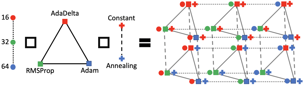
The method constructs the combinatorial graph from the discrete variables, by modelling the variables in a graph depending on the properties of the discrete variables (considering ordinal or categorical). A GP surrogate model is defined over the graph using Graph Fourier Transforms, specifically it uses ARD diffusion kernel to get around the intractability of computing the eigensystem from the graph.
The model works by first considering a ordered sub-graph for every ordinal variable and complete sub-graph for every categorical variable. Then, the cartesian product is computed over the sub-graphs. An illustration is given below. Then a kernel is defined over the graph structure using Graph Fourier Transforms (GFT).
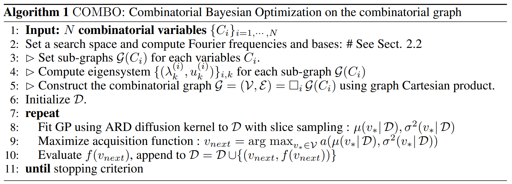
 The next best $x$ is found by the following procedure:
- Evaluating 20000 randomly selected vertices.
- 20 vertices with highest acquisition values are used as initial points for acquisition function optimization.
- Exploring acquisition values on adjacent vertices, the exploration continues recursively on the adjacent vertices until no neighbours' acquisition values are higher than at the current vertex. (Breadth-first local search)
The full algorithm is given below:
GFT can represent any graph signal as a linear combination of graph Fourier bases.
Significance
- Performs implicit variable selection
- Natural metric using Hamming distance on categorical spaces.
- Able to scale to higher dimensions using ARD kernel
Limitations
- Modelling is focused on fully discrete case
- Unnatural metric using Hamming distance on ordinal spaces
Comments
Unnatural metric using Hamming distance on ordinal spaces, which should be modelled using a continous distribution instead. There will be much power that can be unlocked by considering continous distribution. The categorical spaces approach is correct, but not ordinal. Using GFT, maybe there would be some penalty, question is what is the penalty if it exist?
BOCS
The technique used is similar to the discrete part of MiVaBO; they have used second order modelling of the interactions which according to some papers produce a good trade off between expressiveness and the ease of training. The technique uses sparse Bayesian linear regression, instead of GPs. Finding the next best $x$, it finds an approximate optima, considering regularization.
The model works by using linear regression, shown below. In the paper they are careful to account for regularization, by sampling model parameters from the posterior over $\alpha$ and $\sigma^2$ (Noise). $$ f_{\alpha}(x) = \alpha_0 + \sum_j{\alpha_j x_j} + \sum_{i,j>i}{\alpha_{i,j}x_i x_j} $$ For acquisition function, they find the bext best $x$ by solving the following. Note that $\lambda P(x)$ is for regularization; it can be defined differently to achieve different goals. In BOCS, the authors used the L1 Norm $||x||_1$ (another possible definition is L2 Norm). By expanding $P(x)$, we can solve a simple binary quadratic program of the expanded form. $$ \arg\max_{x\in D} {f_{\alpha}(x)} - \lambda P(x) $$
Significance
- Able to control the trade off between expressiveness and ease of training, mainly due to setting of 2nd order of interactions.
- Able to handle sparse data
Limitations
- (Comment from COMBO) Requires users to specify the highest order of interactions among categorical variables (Any higher order interactions are ignored), which restrict its applications to problems with low order interactions between variables
- (Comment from COMBO) Parametric nature of the surrogatre model having excessively large number of parameters.
- Model is inherently designed to be binary Variables only.
BO-Tree Struct
The method models the dependencies of the variables in the program into a decision tree, resulting from the insight that conditional dependencies between hyperparameters can be exploited. The method is tractable as there is a weight vector that would allow the model to couple inference for some paths but still be able to scale to higher-dimensionality. It introduce smoothness by using GPs at the leafs. The optimization to get the next $x$ is done by performing optimization to find the best path then finding the best $x$ on that path.
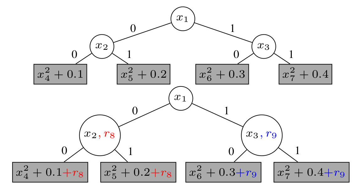
The model works by using linear functions $c^Tr$: $$ y_i \sim N(g_{p_i}(x_i)+z_{p_i}^T c, \sigma^2)\\ c\sim N(0,\Sigma_c)\\ g_p(.)\sim GP $$ Here, $c$ is a weight matrix applied on the feature vector $r$ and $z$ is a binary mask that activates the weights if the inner node decision variables on the path to leaf node $p$. $r$ is used to encode both numerical and categorical parameters. The acquisition function is performed efficiently by using 2 steps, first finding the best path: $$ p_* = \arg\max_{p\in P} \alpha\left(p\mid D_n\right) $$ Then, using $p_*$, find the next best $x$. $$ x_* \in \arg\max_{x\in X_{p_*}} \alpha\left(x,p_*\mid D_n\right) $$
An illustration of functions with tree-structured conditional relationships. Each inner node is a binary variable, and a path in those trees represents successive binary decisions. The leaves contain univariate quadratic functions that are shifted by different constant terms.
Significance
- Allows explicit setting of $c$, to allow the method to use some prior domain knowledge, so that the conditional relationships can be efficiently encoded. (ie. when $c=0$, it can be seen as an independent model, or we can define a prior for $c$)
- Flexible on how the path and kernel can interact, can be changed to use other definitions.
Limitations
- Fundamentally linear interactions, but can be extended. But not both?
- Acquisition function can be intermediate, between what is proposed, vs: $$ (x_*, p_*) \in \arg\max_{p\in P, x\in X_{p}} \alpha\left(x,p\mid D_n\right) $$
The interactions type are standard, which means its either linear or nonlinear interactions. There cannot be a setting that get both.